

Type two distant places into Google Maps and a route can appear in seconds. That feels ordinary only because we see it every day. From a computer-science perspective, it is a remarkable problem: a navigation system has to reason over an enormous road network, account for different road costs and restrictions, incorporate changing traffic conditions, estimate arrival times, and still respond quickly enough to feel instantaneous.
The viral phrase “Google Maps is unreasonably fast” captures that surprise well. But the interesting question is more precise:
How can Google Maps determine a useful route through a huge road network so quickly without checking every possible route?
The answer is not one magic algorithm. Modern routing is a layered engineering problem involving graph representations, shortest-path algorithms, goal-directed search, bidirectional search, preprocessing, hierarchical shortcuts, rapidly updated road costs, traffic prediction, and route-ranking systems.
There is also an important boundary to keep in mind from the beginning: Google does not publicly disclose the complete production routing algorithm used by Google Maps. We can explain the computer science that makes world-scale route planning possible, and we can describe what Google has publicly confirmed about traffic and route selection, without pretending that Dijkstra, A*, or contraction hierarchies are Google’s exact proprietary implementation.
Quick answer
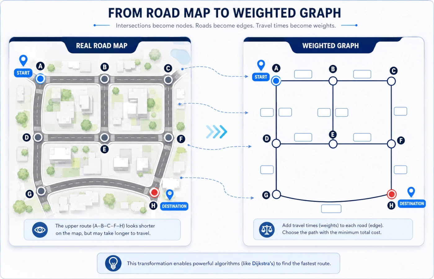
Google Maps does not calculate a route by trying every possible sequence of roads. Modern route planners model a road network as a weighted graph: intersections or road states become nodes, road segments become edges, and each edge receives a cost such as travel time.
Classical algorithms such as Dijkstra’s algorithm can find exact shortest paths, while A* can guide a search toward the destination when a useful lower-bound estimate is available. At continental scale, practical routing systems can go much further by exploiting the hierarchy of road networks and by preprocessing relatively stable information so a live query has to explore only a tiny fraction of the graph.
For Google Maps specifically, Google has publicly confirmed that routing uses current and historical traffic information, machine-learning traffic predictions, road characteristics, restrictions, incident information and other route-quality signals. Google has not publicly documented the complete shortest-path engine behind the consumer product.
Want to see the difference? Race Dijkstra, A*, BFS and bidirectional search on the same synthetic road network with the interactive Route Algorithm Explorer.
When to use this explanation
This article is for you if you are asking questions such as:
- How does Google Maps determine the fastest route?
- How can Google Maps calculate a long route so quickly?
- Does Google Maps use Dijkstra’s algorithm?
- Does Google Maps use A*?
- Does Google Maps use AI for routing?
- How does live traffic change the route?
- Why can Google Maps choose a route that is not simply the shortest by distance?
This is not an article about the Google Maps speedometer, GPS speed accuracy, offline maps, data usage, Google Maps versus Waze, or how to use the Google Maps API. Those are separate search intents.
Before you start
Three ideas make the rest of the article much easier to understand:
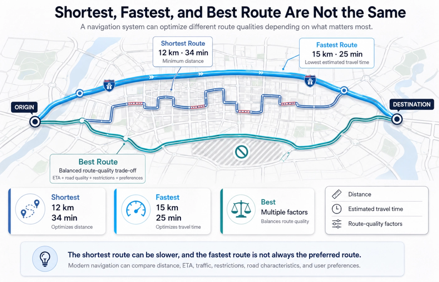
- “Fastest” is not the same as “shortest.” A 12 km route can take longer than a 15 km route.
- A road map can be represented mathematically as a graph. That lets routing become a shortest-path or minimum-cost problem.
- The algorithms described below are a toolkit used in route-planning research and software. They should not be mistaken for a public specification of Google’s private production system.
No programming or advanced mathematics is required. The goal is to build an accurate mental model first, then add the technical details.
Main explanation: the trick is to avoid searching almost everything
Imagine a road network as a giant maze with millions of intersections. A naive approach might try to list every possible route from the start to the destination and then compare them.
That fails almost immediately.
At each intersection there may be several choices. Each of those choices leads to more choices, which lead to still more choices. The number of possible walks through the network grows combinatorially. The source video behind the current trend uses a deliberately simplified New York-to-San Francisco example to illustrate how absurdly large the space of possible routes can become.
The precise number is less important than the lesson:
The speed of a modern route planner comes from proving that most possibilities never need to be examined.
This is the central idea connecting Dijkstra, A*, bidirectional search, road hierarchies and contraction-based routing.
How route planning works, step by step
1. Turn the road map into a weighted graph
A navigation system first needs a mathematical representation of the road network.
At a simplified level:
intersection or road state = node
road segment               = edge
cost of using that segment = weight
A tiny network might look like this:
        4 min
A ───────────── B
│               │
│ 2 min         │ 3 min
│               │
C ───────────── D
        1 min
If you want to travel from A to D, the geometrically shortest-looking route is not automatically the best one. What matters is the sum of the edge weights along the route.
For driving, an edge weight might represent estimated travel time. In a more general routing system, the cost can also reflect restrictions, tolls, turn penalties, road type or other preferences.
This graph abstraction is extremely powerful because the same mathematics works whether the network has four nodes or tens of millions.
2. Reject brute force: do not enumerate every route
The most obvious algorithm is also the worst idea: generate every possible route and choose the cheapest.
Real road networks contain cycles. You can turn around, loop through blocks, enter and leave highways, and create an astronomical number of possible walks. Even after excluding obviously pointless loops, the number of plausible alternatives is far too large for exhaustive enumeration.
A useful route planner therefore needs a stronger question than:
“What routes exist?”
It needs to ask:
“Which parts of the graph can still possibly lead to a better answer?”
Every major acceleration technique in this article is, in one form or another, a better way to answer that second question.
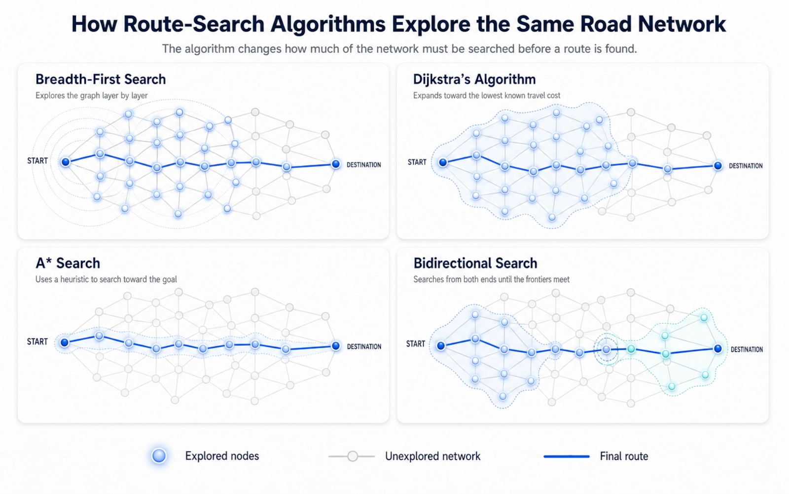
3. Breadth-first search shows the basic search idea
For an unweighted graph, breadth-first search (BFS) is a natural starting point.
It expands the graph layer by layer:
start
  ↓
all nodes 1 step away
  ↓
all nodes 2 steps away
  ↓
all nodes 3 steps away
  ↓
...
If every edge has the same cost, the first time BFS reaches the destination it has found a path with the minimum number of edges.
Roads do not behave like that. One road segment may take 30 seconds, another 10 minutes. A highway edge and a congested city street should not count as equal just because each is “one edge.”
That is why weighted road networks lead naturally to Dijkstra’s algorithm.
4. Dijkstra explores routes in increasing cost order
Edsger W. Dijkstra devised his shortest-path method in 1956 and published it in 1959 in Numerische Mathematik.
The core idea is elegant:
- Give the starting node a cost of
0. - Give every other node an initial cost of infinity.
- Choose the unexplored node with the lowest known cost.
- Try to improve the costs of its neighbours.
- Once the cheapest unexplored node is finalized, continue with the next cheapest one.
- Stop when the destination is finalized.
Conceptually:
known cost so far
        ↓
expand the cheapest frontier node
        ↓
update neighbouring costs
        ↓
repeat
If all edge weights are non-negative, Dijkstra’s algorithm can guarantee an optimal shortest path.
That guarantee is why Dijkstra remains foundational.
But there is a scaling problem.
Why Dijkstra can search far too much
Dijkstra does not inherently know which direction the destination lies in. It searches outward according to accumulated cost.
If your destination is east, it can still explore many roads north, west and south because those roads may initially be cheap enough that they cannot yet be ruled out.
The source video’s OpenStreetMap-based experiment illustrates this nicely. In a Newark Airport-to-Central Park Zoo test, a Dijkstra search visited more than 65,000 nodes and still completed in roughly a tenth of a second on that test setup. That is impressive—but the amount of unnecessary search becomes much more serious as the graph and route length grow.
For a large continental network, “plain Dijkstra for every request” is not the engineering endpoint.
5. A* points the search toward the destination
A* adds a second ingredient to the cost used for prioritizing nodes.
Dijkstra effectively considers:
g(n) = cost from start to node nA* considers:
f(n) = g(n) + h(n)where:
g(n)is the known cost from the start to noden;h(n)is an estimate of the remaining cost fromnto the destination.
The heuristic h(n) acts like a compass. Instead of expanding equally promising nodes in every direction, A* can prefer nodes that also appear closer to the goal.
A useful mental picture is:
Dijkstra:
        ↖ ↑ ↗
      ← START →
        ↙ ↓ ↘

A*:
START ───────────────→ DESTINATION
With an admissible heuristic—one that never overestimates the true remaining cost—A* can preserve optimality while reducing the search space.
Why A* is not automatically a complete solution for driving time
For pure geographic distance, straight-line distance is an obvious lower bound: no road route can be shorter than teleporting directly from the current point to the destination.
Travel time is more complicated.
You can convert straight-line distance into a lower-bound time by assuming a very high feasible speed, but that estimate can be weak. It knows nothing about:
- which roads actually exist;
- one-way restrictions;
- bridges and rivers;
- mountains;
- congestion;
- low-speed urban streets;
- turn restrictions.
The safer the heuristic is against overestimating, the less informative it may become.
So A* is a major idea in pathfinding, but large road-network routing can benefit from stronger structural information than “the destination is roughly over there.”
6. Bidirectional search attacks the problem from both ends
Another powerful idea is to search from both the start and the destination.
Instead of:
START >>>>>>>>>>>>>>>>>>>>>>> DESTINATIONa bidirectional search tries to make two smaller searches meet:
START >>>>>>>           <<<<<<< DESTINATION
                    X
Why can that help?
Search spaces often grow rapidly with radius. Replacing one large search radius with two smaller ones can reduce the amount of graph explored dramatically.
On directed road networks, the backward side has to respect directionality correctly—for example by searching an appropriately reversed representation of the graph—but the high-level principle is simple.
Bidirectional search is especially important because it combines naturally with hierarchical routing methods.
Try it yourself: Route Algorithm Explorer
Reading about the search patterns is useful. Watching them compete on the exact same road network makes the difference much easier to see.
Choose a start and destination, add traffic if you want, and run Breadth-First Search, Dijkstra, A*, or bidirectional search.
The explorer shows how many nodes each method expands, how its search frontier grows, which path it finds, and the final path cost.
This is an educational routing simulator. It does not reproduce Google Maps’ proprietary routing system.
Interactive computer-science lab
Route Algorithm Explorer
Pick two intersections. Add traffic. Watch four pathfinding algorithms solve the same synthetic road network.
Try an experiment
Start with a question, not an empty graph
Measured search work
Results
Run an algorithm to see metrics.
Advanced mode
Algorithm internals
Run an algorithm to inspect the frontier and scores.
- Nodes explored
- Nodes removed from the frontier and expanded by the algorithm.
- Frontier
- Discovered nodes that may still be explored.
- Path cost
- The sum of the current edge weights on the final route.
Open the full Route Algorithm Explorer →
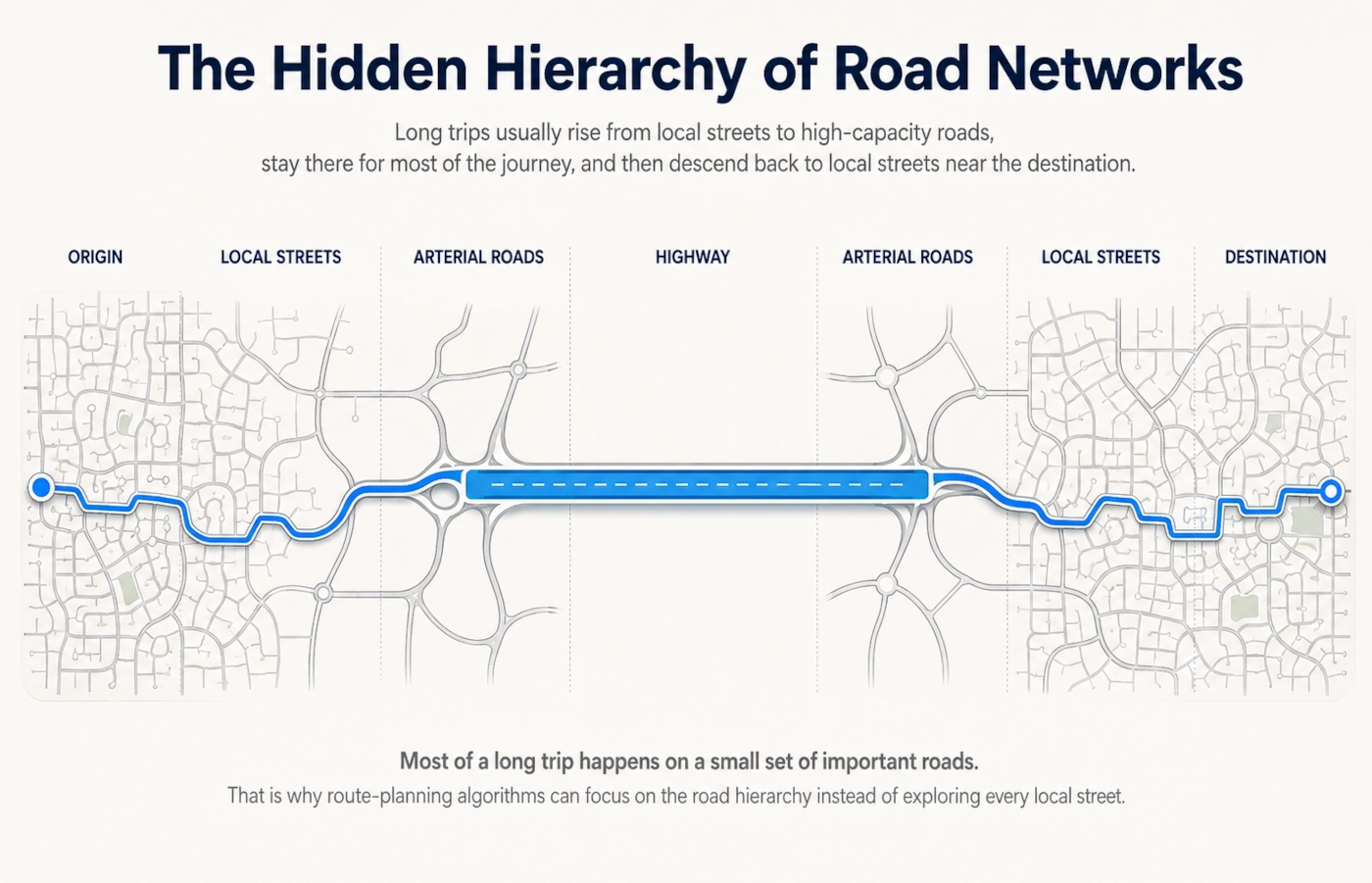
7. Exploit the hidden hierarchy of real road networks
Human drivers already understand a fact that is easy to miss when looking at a raw graph:
Not every road is equally important for a long trip.
A cross-country journey usually has a shape like this:
local street
    ↓
larger local road
    ↓
arterial road
    ↓
highway
    ↓
arterial road
    ↓
local street
    ↓
destination
You do not seriously consider every residential cul-de-sac in every city between your origin and destination.
Real road networks have an inherent hierarchy:
- many roads matter only near the start or destination;
- a smaller set of roads carries regional traffic;
- an even smaller set of corridors and crossings matters for long-distance movement.
A routing algorithm that can exploit this structure has an enormous advantage over a search that treats every junction as equally relevant.
This is where preprocessing becomes transformative.
8. Preprocess stable structure before the user asks for a route
There are two extreme strategies:
Extreme A: no preprocessing
request arrives
    ↓
start from raw graph
    ↓
do almost all the work now
This keeps preparation cheap, but queries can be expensive.
Extreme B: precompute every answer
every possible origin
×
every possible destination
=
massive lookup table
That would make individual queries trivial, but the storage and preprocessing requirements would be enormous, and changing roads or costs would make the table difficult to maintain.
Practical route-planning research looks for a useful middle ground:
Precompute enough structure to make queries tiny, without precomputing every route.
This is the key idea behind several families of road-network speedup techniques.
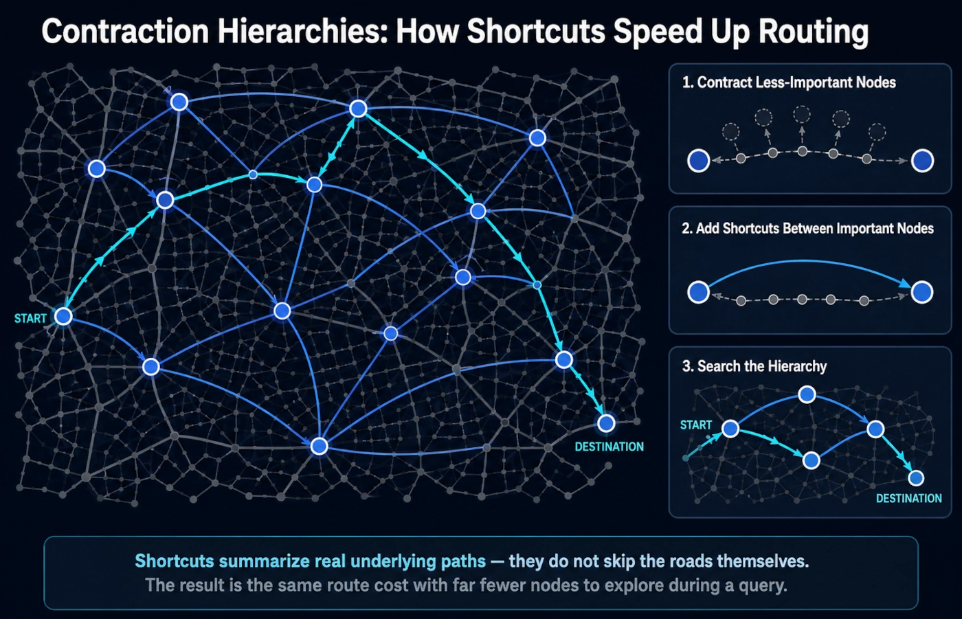
9. Contraction Hierarchies add shortcuts through less important regions
Contraction Hierarchies (CH) are a classic example of preprocessing designed specifically for fast road routing.
The broad idea is:
- Order nodes by importance.
- Contract less important nodes.
- Add shortcut edges when necessary so shortest-path distances are preserved.
- At query time, search mainly upward through the hierarchy.
- Reconstruct the original road sequence from the shortcut path.
Imagine a chain:
A ─ B ─ C ─ D ─ E ─ FIf a precomputed shortcut preserves the cost of travelling through several intermediate nodes, a query can conceptually traverse something closer to:
A ───────── D ─────── Fwithout individually exploring every local node during the live search.
The important point is that shortcuts are not fake teleportation. They summarize real paths while preserving the relevant shortest-path cost.
The 2012 Transportation Science paper “Exact Routing in Large Road Networks Using Contraction Hierarchies” describes CH as exploiting the inherent hierarchy of road networks during preprocessing and then using a modified bidirectional Dijkstra search. In its experiments, the resulting searches could visit only a few hundred nodes on continental road networks.
That is the kind of transformation required for interactive routing: not a 10% improvement, but orders of magnitude less search.
Good hierarchy design matters
Not every contraction order is equally efficient.
A poor ordering may:
- create too many shortcuts;
- consume too much memory;
- leave too much work for the query;
- destroy the benefit of the hierarchy.
A good ordering tries to preserve a sparse graph while identifying structurally important separators and corridors.
10. Customizable Contraction Hierarchies separate topology from changing weights
Standard contraction hierarchies are extremely fast, but live navigation has an awkward property:
The road network is relatively stable, while travel-time weights can change frequently.
A bridge normally stays where it is.
Its travel time may change minute by minute.
That creates two kinds of information:
topology:
which roads connect to which roads
changes relatively slowly

weights:
how expensive each road is right now
can change rapidly
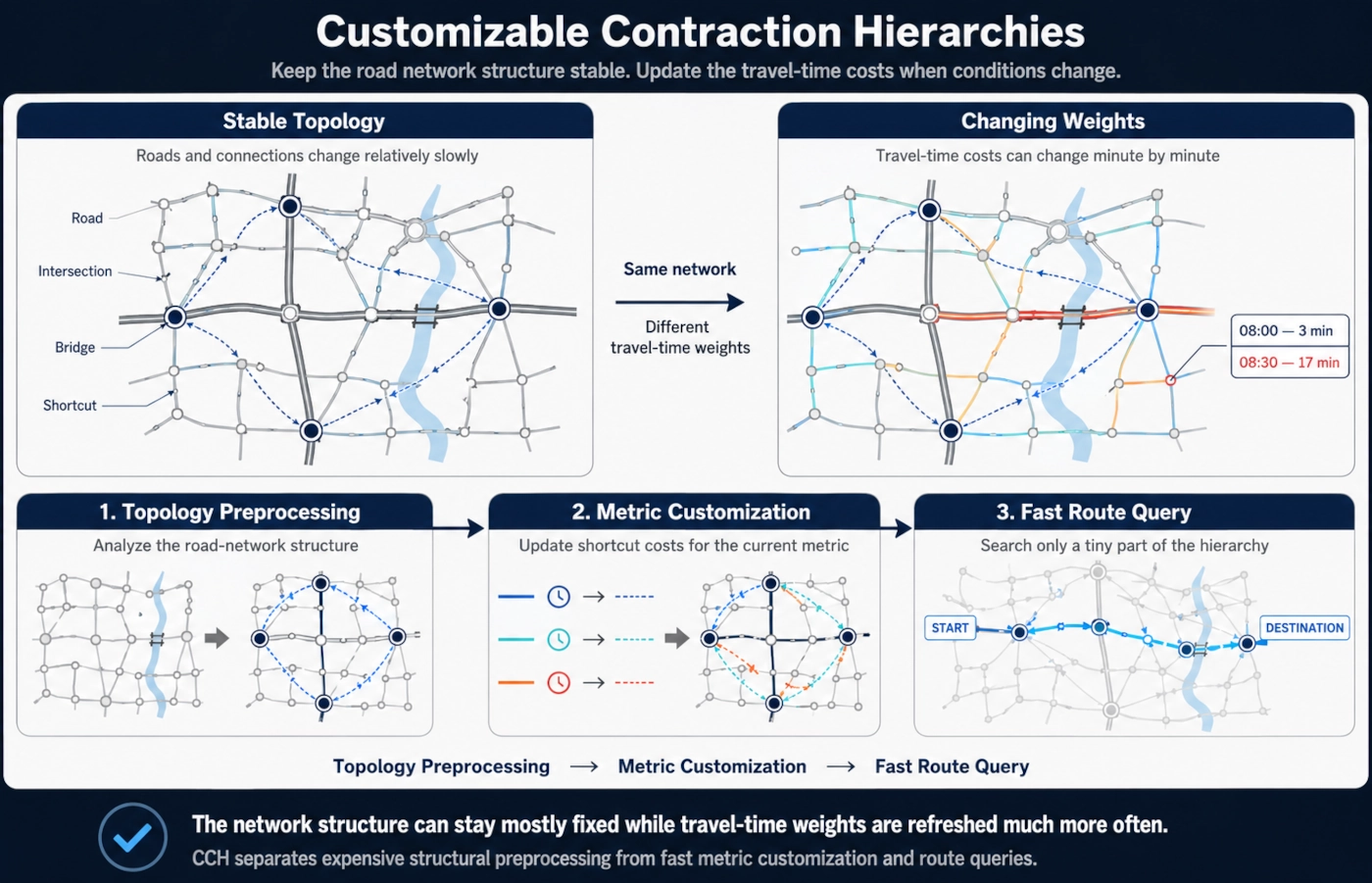
Customizable Contraction Hierarchies (CCH) were designed around this distinction.
The CCH paper describes a three-phase workflow:
- Preprocessing — analyze the unweighted topology and build reusable structural information.
- Customization — adapt the hierarchy to a particular set of edge weights.
- Query — answer origin-to-destination shortest-path requests quickly.
CCH uses nested dissection orders, which seek small graph separators that divide a graph into large pieces. Intuitively, if a small set of crossings connects two huge regions, those crossings are structurally important.
The source video’s North American experiment gives a vivid illustration: a small high-ranked separator roughly followed major Mississippi crossings, reflecting the fact that relatively few road crossings connect large regions on either side.
That is an example from the video’s experimental network, not a claim about Google’s internal graph.
Why customization matters for traffic
Suppose a road has this cost at 08:00:
road A = 3 minutesA crash occurs, and at 08:30 the cost becomes:
road A = 17 minutesThe physical road network did not need to be rediscovered. What changed was the routing metric.
CCH-style designs show how route planning can separate the expensive understanding of network structure from a faster weight-update phase.
Again, this is an important route-planning technique, not proof that Google Maps currently uses CCH.
What the source video’s experiment actually shows
The video that triggered the current query uses real road-network data and custom pathfinding experiments to demonstrate the scale of the speedup that hierarchical preprocessing can produce.
For a long path on its North American network, the experiment reports approximately:
| Method in the experiment | Search behaviour |
|---|---|
| Well-tuned Dijkstra | Explores much of a 64-million-plus-node network; around seconds for a long route |
| Customizable Contraction Hierarchy | Roughly 200 microseconds for the query in the demonstrated setup |
| Average CCH search space | Around 1,450 explored nodes in the demonstrated tests |
The video describes the CCH query as roughly 35,000 times faster than Dijkstra in that particular experiment.
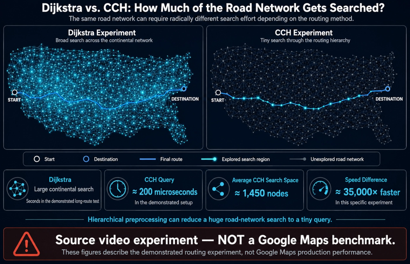
These numbers are useful because they make the scale of hierarchical routing tangible.
They are not Google Maps benchmarks.
Hardware, graph representation, preprocessing quality, cost model, implementation language, memory layout, route length and many other factors affect runtime. The correct conclusion is:
Modern hierarchical route-planning algorithms can reduce a huge graph search to a very small query.
The incorrect conclusion is:
Google Maps itself computes routes in 200 microseconds using CCH.
Google has not published evidence supporting that second statement.
Where live traffic and machine learning enter the picture
Shortest-path algorithms need edge weights.
For a driving route, those weights are closely related to a deceptively hard question:
How long will this road segment take when the driver reaches it?
That is not necessarily the same as:
- its current travel time;
- its speed limit;
- yesterday’s travel time;
- its average travel time.
If a 45-minute trip starts now, the traffic on a road near the destination may be very different 40 minutes from now.
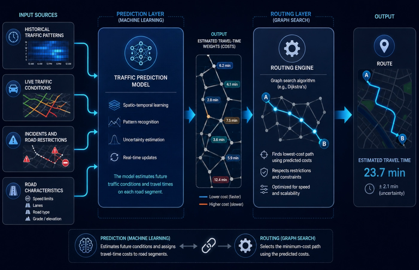
Google has publicly explained that Google Maps combines historical traffic patterns with live traffic conditions and uses machine learning to predict near-future traffic. Google’s 2020 Maps explanation also says predictive traffic models are part of route determination.
A useful conceptual separation is:
routing engine:
Which path has the best cost under the current model?

traffic / ETA models:
What cost should each road have now or when the driver reaches it?
Machine learning can greatly improve the second problem without replacing classical graph search in the first.
That distinction prevents a common oversimplification: saying “AI finds the shortest path” hides several different problems behind one label.
What Google has publicly confirmed about route calculation
Google publishes enough information to establish several important facts.
Google Maps uses traffic-aware routing
The current Google Maps Platform Routes API documentation distinguishes three routing preferences:
TRAFFIC_UNAWARETRAFFIC_AWARETRAFFIC_AWARE_OPTIMAL
Google states that TRAFFIC_AWARE_OPTIMAL considers current traffic, performs a more exhaustive road-network search and is equivalent to the routing mode used by maps.google.com and the Google Maps mobile app.
That is a particularly useful public statement because it confirms that the consumer Maps experience is traffic-aware and that Google explicitly manages a quality-versus-latency trade-off.
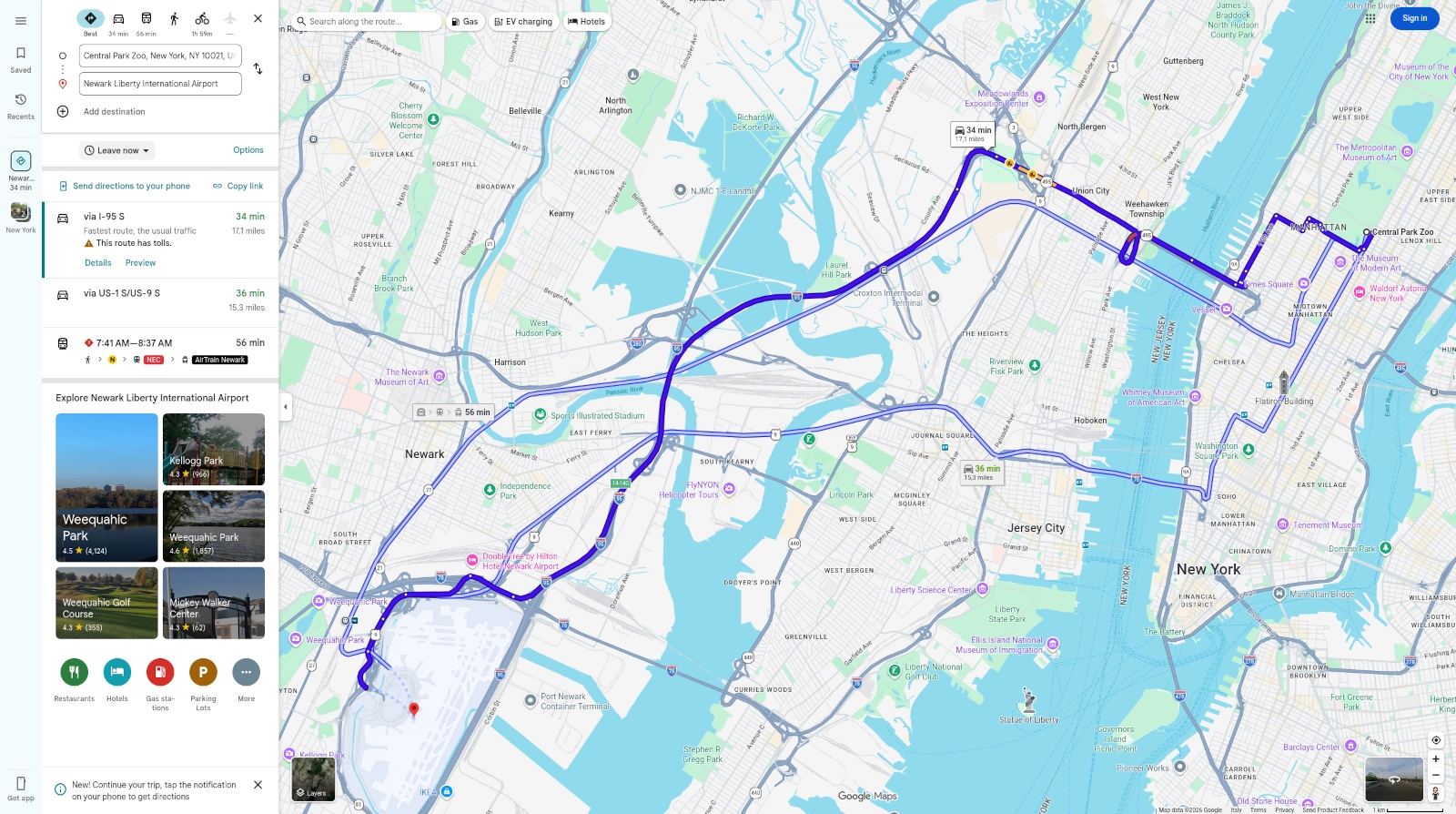
Example Google Maps route options. Travel times and recommended routes change with traffic and other conditions.
Google uses live and historical traffic information
Google has explained that aggregate location data from navigation can help estimate current road conditions, while historical road-traffic patterns are combined with live conditions for prediction.
For future departure times, Google’s Routes API documentation similarly explains that live traffic is weighted more heavily close to the present, while historical conditions matter more as the departure time moves farther into the future.
Google uses machine learning for traffic prediction
Google has publicly described machine-learning systems used to improve traffic and ETA predictions, including work with DeepMind on graph neural networks.
That helps answer the query “Does Google Maps use AI?”
Yes—but “Google Maps uses AI” is not the same statement as “Google Maps uses an AI model instead of shortest-path algorithms.”
Traffic forecasting, ETA estimation, map understanding and route preference are different subproblems.
Google can optimize for more than raw ETA
Google Research describes route recommendation as a trade-off involving factors such as:
- estimated time of arrival;
- tolls;
- route directness;
- road surface conditions;
- user preferences;
- transportation mode;
- local geography.
Google’s own Maps explanation also discusses road quality, road size and directness, restrictions, government data and incident reports.
So the consumer-facing phrase “best route” is more accurate than assuming that route selection is always a single mathematical race for the lowest current ETA.
Shortest route, fastest route and best route are different
These three phrases are often treated as interchangeable. They are not.
Shortest route
Minimizes physical distance.
Route A: 12 km
Route B: 15 km

Shortest = Route A
Fastest route
Minimizes estimated travel time.
Route A: 12 km, 34 min
Route B: 15 km, 25 min

Fastest = Route B
Best route
May balance several costs or preferences.
A route can be less attractive despite a similar ETA if it involves factors such as:
- tolls;
- awkward local roads;
- an unpaved surface;
- restrictions;
- predicted congestion;
- undesirable route characteristics.
This is one reason a navigation app may appear to “ignore” a route that looks faster or shorter to a human looking at the map.
The map is not necessarily optimizing the same single quantity you are eyeballing.
Why Google Maps can change your route while you are driving
A route is not a permanent answer.
It is the best answer under a model of the network at a particular time.
During the drive, several inputs can change:
- traffic slows down;
- a crash is reported;
- a lane or road closes;
- a restriction changes;
- the driver’s progress changes;
- a predicted future bottleneck becomes more or less likely;
- an alternative route becomes better under updated costs.
Conceptually:
08:00
Path A = 32 min
Path B = 37 min
→ choose A

08:12
new congestion on A

Path A = 45 min
Path B = 34 min
→ B may now be preferable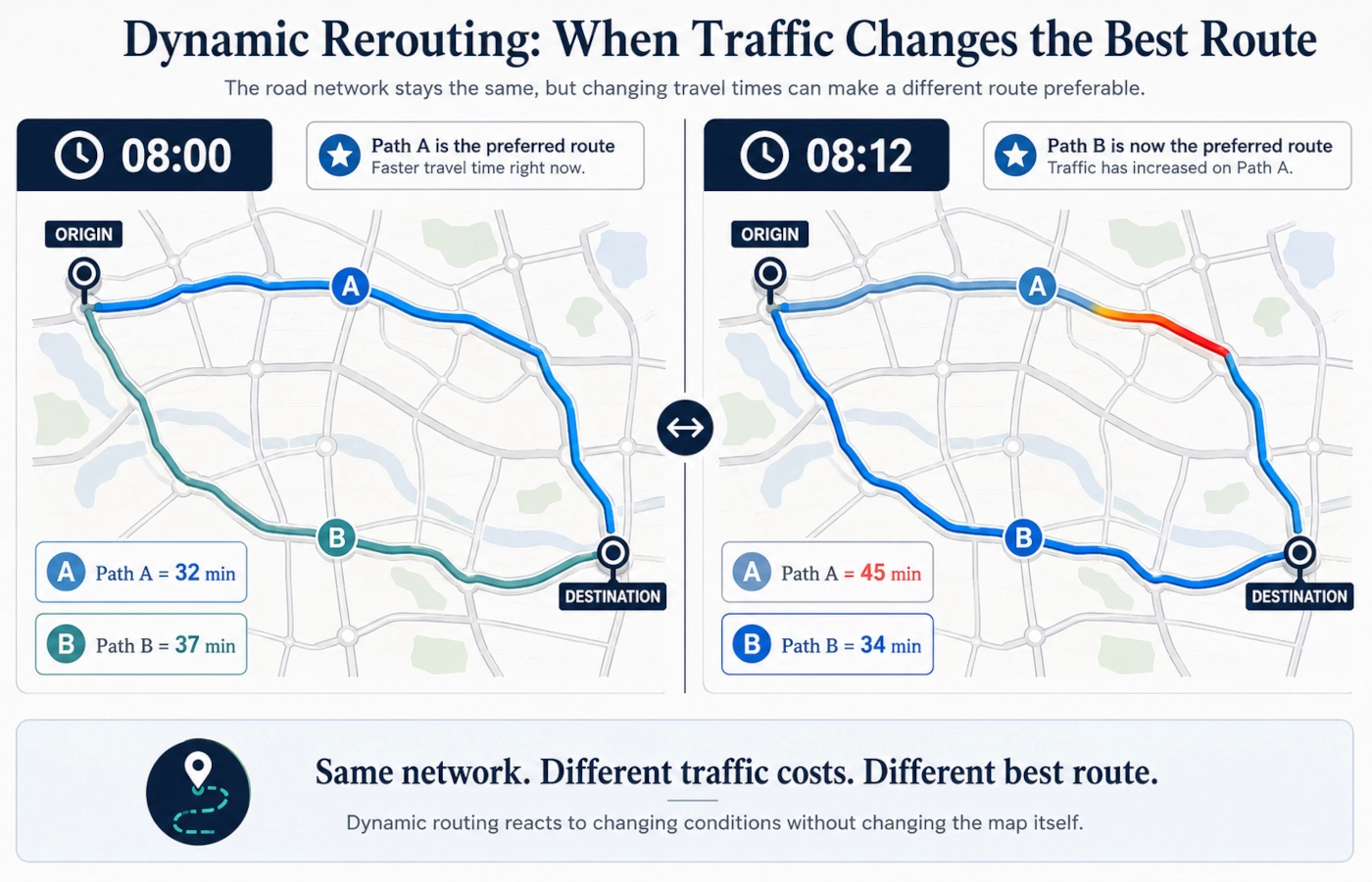
A navigation system can therefore rerun or update route calculations as the relevant costs change.
The important engineering challenge is to make these repeated decisions fast enough that recalculation feels immediate.
Does Google Maps actually use Dijkstra, A*, or contraction hierarchies?
This is where many explanations become too confident.
Dijkstra
Dijkstra’s algorithm is foundational to shortest-path computation on graphs with non-negative edge weights. Many later routing techniques build on ideas from Dijkstra or compare themselves against it.
That does not prove that today’s Google Maps consumer routing request is simply running textbook Dijkstra over the full global road graph.
A*
A* is a foundational goal-directed search technique. With a good admissible heuristic, it can dramatically reduce the amount of graph explored while preserving optimality.
That does not prove that Google’s current production route engine is textbook A*.
Contraction Hierarchies
Contraction Hierarchies are specifically designed to accelerate shortest-path queries in large road networks through preprocessing, hierarchy and shortcuts. Their academic performance demonstrates why enormous road graphs can be searched far faster than raw Dijkstra would suggest.
That does not prove Google Maps uses CH.
Customizable Contraction Hierarchies
CCH extends the idea by separating topology preprocessing from fast metric customization, making it especially relevant when edge weights change.
That does not prove Google Maps uses CCH.
The correct conclusion
We can explain how modern routing can be this fast without claiming to know Google’s proprietary routing stack.
That is both more accurate and more useful.
What we know vs. what we do not know
| Publicly supported | Not publicly established |
|---|---|
| Google Maps uses traffic information | Google’s exact production shortest-path algorithm |
| Google combines historical and live traffic for prediction | Whether consumer Maps currently uses textbook Dijkstra |
| Google uses machine learning in traffic and ETA systems | Whether consumer Maps currently uses textbook A* |
| Google Maps performs traffic-aware routing | Whether Google currently uses CH or CCH |
| Google route recommendation can consider multiple factors | Google’s complete graph representation and data structures |
| Google manages route-quality versus response-latency trade-offs | Every proprietary heuristic and optimization |
| Modern routing research can answer huge road-network queries extremely quickly | Google’s internal per-query node count or microsecond runtime |
This distinction is one of the most important parts of understanding the topic correctly.
Why Google Maps feels “unreasonably fast”
The answer is now easier to see.
Google Maps is not solving the problem you first imagine.
It is not:
user asks for route
    ↓
generate every possible path
    ↓
compare all paths
    ↓
return winner
A modern system can instead behave conceptually more like:
maintain a structured road graph
        ↓
precompute useful structural information
        ↓
continuously estimate or update road costs
        ↓
receive start + destination
        ↓
search a highly constrained portion of the network
        ↓
evaluate route quality using current predictions/preferences
        ↓
return route
        ↓
re-evaluate when conditions change
The live request is therefore the final stage of a much larger system.
A great deal of work has already happened before you tap Directions.
Try the experiment yourself: change the start, destination or traffic costs in the Route Algorithm Explorer and see how dramatically the explored search space changes.
Common mistakes
Mistake 1: “Google Maps checks every possible route”
It does not need to.
Exhaustive route enumeration is exactly what scalable graph algorithms are designed to avoid.
Mistake 2: “Google Maps uses Dijkstra, full stop”
That statement is too strong.
Dijkstra explains a foundational shortest-path method. It does not reveal Google’s private production implementation.
Mistake 3: “A* is always faster than Dijkstra”
Not necessarily.
A* gains its advantage from its heuristic. With an excellent heuristic it can search far less. With a weak heuristic, its behaviour approaches Dijkstra. Dijkstra can be viewed as the special case where the heuristic is zero.
Mistake 4: “The shortest route is the fastest route”
Distance and time are different cost functions.
Traffic, road type, turns and restrictions can make a longer route faster.
Mistake 5: “Machine learning replaced graph algorithms”
Google uses machine learning in traffic prediction and route-related systems, but that does not mean classical graph optimization became irrelevant.
Prediction and path search solve different parts of the problem.
Mistake 6: “The 200-microsecond experiment is Google Maps performance”
It is not.
That result comes from the source video’s CCH experiment on its own setup. It is evidence about what modern routing techniques can achieve, not a benchmark of Google’s infrastructure.
Mistake 7: “A route should never change after it is calculated”
Traffic-aware edge costs can change. Re-routing is a feature of a dynamic navigation system, not proof that the first calculation was broken.
Security, privacy and safety notes
Route-planning algorithms and traffic-data systems should not be conflated with assumptions about what personal data Google stores about a particular user.
Google’s public explanation states that aggregate location data can be used to understand traffic conditions. This article does not attempt to reverse-engineer Google’s user-level data handling, retention or privacy settings.
For privacy controls, account history and location settings, use Google’s current privacy documentation rather than inferring policy from routing behaviour.
For driving safety, a mathematically preferred route is not permission to ignore:
- road signs;
- temporary closures;
- local laws;
- police or emergency directions;
- real-world hazards;
- conditions that are not yet reflected in the map.
Navigation is decision support. The driver remains responsible for following the road safely and legally.
Faster alternative
If you only want the 30-second mental model, remember these three layers:
- Graph search: roads become a weighted graph, so algorithms can find low-cost paths without enumerating every route.
- Acceleration: preprocessing, hierarchy and shortcuts can reduce a continental search to a tiny fraction of the network.
- Dynamic intelligence: traffic prediction and other route-quality signals continuously change the costs and ranking of candidate routes.
That model is deliberately simplified. It gives you the central idea without the details of A*, bidirectional search, contraction hierarchies or customization.
FAQ
How does Google Maps determine the fastest route?
At a high level, Google Maps uses a digital road network together with travel-time estimates, current and historical traffic information, restrictions and other route-quality signals. Google publicly documents traffic-aware routing and machine-learning traffic prediction, but it does not publish the complete production shortest-path algorithm used by the consumer product.
Does Google Maps use Dijkstra’s algorithm?
Dijkstra is a foundational shortest-path algorithm and an important way to understand route planning. Google has not publicly documented the current consumer Google Maps routing engine in enough detail to say that every route request is solved by textbook Dijkstra.
Does Google Maps use A*?
A* is a major goal-directed pathfinding algorithm and is highly relevant to route-planning theory. There is not enough public information to state that today’s Google Maps consumer routing system uses textbook A* as its exact production algorithm.
Is A* faster than Dijkstra?
Often, but not automatically. A* can explore far fewer nodes when it has a strong heuristic. If the heuristic provides little useful information, A* approaches Dijkstra’s behaviour. Performance also depends on implementation, graph structure and the cost metric.
Does Google Maps use contraction hierarchies?
Google has not publicly confirmed that the current consumer Maps product uses Contraction Hierarchies or Customizable Contraction Hierarchies. These algorithms are important because they demonstrate how preprocessing and road-network hierarchy can make exact routing on very large graphs extremely fast.
Does Google Maps use AI to calculate routes?
Google uses machine learning for traffic and ETA prediction and has published research on learning route preferences. That does not mean an AI model simply replaces shortest-path graph algorithms. Route planning is a pipeline containing multiple optimization and prediction problems.
How does Google Maps predict traffic?
Google has explained that it combines historical traffic patterns with live traffic conditions and uses machine learning to predict how traffic may develop during a trip. Current Google Routes documentation also distinguishes between live and historical traffic depending on routing mode and departure time.
Why doesn’t Google Maps always show the route that looks fastest to me?
Because the route that looks shortest on the map may not have the lowest predicted travel time, and Google’s route recommendation can consider more than ETA alone. Public Google research discusses factors including tolls, directness, road surface and user preferences.
Does Google Maps calculate every possible route?
No scalable route planner would need to enumerate every possible route. Shortest-path algorithms eliminate possibilities systematically, and modern road-routing methods can use preprocessing, hierarchy and shortcuts to reduce the live search dramatically.
How quickly can modern routing algorithms find a path?
It depends on the graph, hardware, cost model and preprocessing. Academic contraction-hierarchy research reports sub-millisecond-style query performance on large road networks in experimental settings. The source video’s CCH demonstration reports roughly 200 microseconds for its particular setup. Neither figure should be interpreted as a Google Maps production benchmark.
What is the difference between the shortest route and the fastest route?
The shortest route minimizes distance. The fastest route minimizes estimated travel time. They can be different because roads have different speeds, congestion, turns, restrictions and conditions.
Why can Google Maps change routes while I am driving?
Because the cost of roads changes. New traffic, incidents, closures and updated predictions can make another route preferable. A traffic-aware navigation system can recalculate as those inputs change.
Sources and further reading
For readers who want to go beyond the simplified explanation, these are the most useful primary and official sources:
- Google Maps 101: How AI helps predict traffic and determine routes — Google’s explanation of live traffic, historical patterns, machine learning and route selection.
- Google Maps Platform Routes API: Set the level of traffic data — current documentation on traffic-aware routing, quality-versus-latency trade-offs and the mode equivalent to Google Maps web/mobile.
- World scale inverse reinforcement learning in Google Maps — Google Research on learning route preferences at world scale.
- A note on two problems in connexion with graphs — Dijkstra’s 1959 paper.
- A Formal Basis for the Heuristic Determination of Minimum Cost Paths — the foundational A* paper by Hart, Nilsson and Raphael.
- Exact Routing in Large Road Networks Using Contraction Hierarchies — technical treatment of exact routing with contraction hierarchies.
- Customizable Contraction Hierarchies — the topology/customization/query approach and nested-dissection-based ordering.
- Google Maps is unreasonably fast. Let me explain — the Veritasium and 2swap video whose experiments motivated the current search trend and several examples discussed above.
Last tested
Tested/reviewed against:
- Google Maps web route planner
- Google Maps mobile app routing behaviour
- Google Maps Platform Routes API documentation
- Google Research routing publications
- Dijkstra, A*, Contraction Hierarchies and Customizable Contraction Hierarchies primary literature
Last tested: 2026-08-14
Related guides
Carefully selected guides to help you understand the topic and complete the next useful step.